Inside the Commander: What It Sees and What It Decides

The previous post ended on a claim I owe you evidence for: that getting the reward function right was the hardest part of this project. Before I can show you that, I have to show you what the Commander is actually working with — what it can see, and what it is allowed to do about it. Those two things bound everything the reward function can possibly ask for.

The Commander never directly touches a replica count. It does not know how many pods service X is running. All it does is answer one question: how should I distribute the cluster’s capacity across five domains, right now, given what I know and what I expect?

This post is the mechanics: the observation vector, the action space, and the handful of places where the infrastructure underneath leaks into both. The reward function — where I made most of my mistakes — comes next.

What the Commander Sees

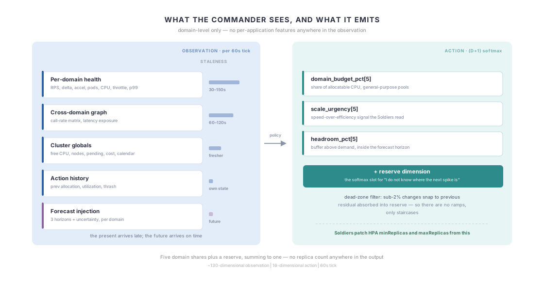
The Commander’s observation vector is a concatenation of per-domain aggregates. Five domains, each contributing a block of features:

Per domain (×5):
  traffic_rps_current          # Current aggregate RPS
  traffic_rps_p95_15m          # 95th pct RPS over last 15 min
  traffic_rps_delta            # Change vs previous tick
  traffic_rps_acceleration     # Distinguishes sharp-onset from gradual spikes
  pod_count_current            # Live pods
  pod_count_pending            # Pods in Pending state
  cpu_utilization_p75          # p75 of per-workload CPU-vs-request ratio
  cpu_throttled_pct            # CFS throttling — a p99 driver that mean CPU is blind to.
                               #   Only non-zero where CPU limits are set, so this partly
                               #   measures which teams set limits.
  memory_utilization_p75       # Domain-wide memory p75
  latency_p99_ms               # Merged-histogram p99 across the domain's workloads
  pod_restart_rate_5m          # Restarts per minute (paired with CrashLoopBackOff count,
                               #   which does not saturate under exponential backoff)
  slo_headroom_pct             # 1 - (latency_p99 / latency_slo) — normalized proximity
                               #   to breach. Trailing, not leading.

Cross-domain dependency signals (Istio, aggregated to domain pairs by a recording
rule filtered to reporter="destination" — both proxies report every call, and
summing without that filter doubles the entire matrix):
  cross_domain_call_rate[D×D]  # Inter-domain RPC rate matrix — tells the Commander
                               #   which domains are coupled (e.g., Payment → Fraud)
  cross_domain_latency_exposure[D]  # Call-share-weighted exposure to upstream degradation:
                               #   Σ_{d'≠d} (call_rate[d→d'] / Σ call_rate[d→·])
                               #            × max(0, latency_p99[d']/latency_slo[d'] - 1)

Cluster globals:
  cluster_cpu_available_pct    # Free allocatable CPU in the shared pools
  cluster_node_count           # Current node count
  cluster_node_pending_count   # Nodes being provisioned
  cluster_cost_per_min         # Rolling cost (from node types/counts, not billing API — expect noise)

Temporal context (also fed to the forecaster as known-future covariates):
  hour_of_day
  day_of_week
  is_special_event_flag        # Promotion, major deployment, etc.

Action history and feedback:
  prev_budget_allocation[D]    # Commander's own previous budget allocation
  soldier_budget_utilization[D]# How much of allocated budget each Soldier actually used
  rolling_thrash_count[D]      # Node provision events over the last 10 min, split
                               #   fractionally across domains by their share of the
                               #   pending pods that triggered each one. Noisy, and
                               #   blind to the deprovision half.

Injected from forecaster (5 domains × 3 horizons, plus one uncertainty scalar per domain):
  traffic_forecast_p80_t5m[D]
  traffic_forecast_p80_t15m[D]
  traffic_forecast_p80_t30m[D]
  forecast_uncertainty[D]      # (p90-p10)/p50 at t+15m

Two of those were not in the original design. traffic_rps_delta and traffic_rps_acceleration were added after shadow mode, once it was clear the policy could not distinguish a sharp-onset spike from a gradual ramp from level signals alone. Adding them meant re-running training from Stage 2 — you cannot widen an input layer on a trained network — which is the kind of cost that makes you think hard before adding a feature. The debt that remains is subtler: the simulator’s generative model for those two signals was fitted after the fact, to shadow-mode data, rather than being part of the original calibration. Every other input was validated against production traces before the policy ever saw it. These two were not.

What the Commander actually sees, and when. None of this is live. At 100k pods the collection pipeline imposes real lag, and it is the same order of magnitude as the lead times the Commander is trying to buy:

So the CPU signal driving a 60-second decision describes the cluster one to two and a half ticks ago. The forecaster covers exactly one row of that table — traffic — and nothing else in it. For the rest, the mitigation is cruder: the 60-second tick was set to roughly the same order as the lag, on the theory that a controller which cannot see faster than it acts is at least not fooling itself. The Commander is always reasoning about a stale present and a probabilistic future, never about now.

The Soldiers have it worse, and this is the part I underrated for a long time. They tick every ten seconds against the same pipeline. Two ticks in every three see byte-identical inputs, and all of them see a cluster somewhere between thirty seconds and two and a half minutes old. A ten-second control loop on ninety-second telemetry is not really a ten-second control loop. It is a sixty-to-ninety-second loop that samples six times as often, and the extra samples buy nothing except a faster path to acting on noise.

One pipeline detail that matters more than it sounds: Istio’s default latency histogram buckets jump 100 → 250 → 500ms, so a p99 near a 150ms SLO lands mid-bucket and carries tens of milliseconds of interpolation error. A reward function with a carefully shaped gradient near the SLO boundary is worthless if the telemetry cannot resolve that boundary. I had to define custom buckets clustered around each domain’s SLO before any of the reward shaping in the next post meant anything.

The deliberate design choice here is what is absent: there are no per-application features in the Commander’s observation. The Commander has no idea how many replicas service X is running or what its CPU looks like. That information lives entirely in the Soldiers’ observation space.

That constraint is load-bearing. The Commander’s tractability comes from operating at domain-level abstraction. If I added per-app features, I would be back to the dimensionality problem that killed the monolithic agent approach.

What the Commander Decides

The Commander’s actor outputs a budget directive per domain. Concretely (field names simplified from the architecture doc for readability):

action = {
    domain_budget_pct[5],    # Share of allocatable CPU in the shared node pools
    scale_urgency[5],        # Urgency signal 0–1 (Soldiers read this)
    headroom_pct[5],         # Buffer above current demand (not above forecast —
                             #   forecast already uses p80 CI; this covers demand
                             #   variability within the forecast horizon)
}

A note on units, because “percentage of cluster capacity” is ambiguous enough to be meaningless: budget percentages are shares of allocatable CPU in the general-purpose node pools, with memory tracked as a secondary binding constraint. One percentage point of that contested pool is on the order of 750 pods at current density — the whole cluster is around 100k, but a meaningful slice of Fraud’s inference tier and most of Data Pipelines’ batch capacity live on dedicated pools the Commander cannot reach. This is also one cluster, not a fleet: 100k pods sits under Kubernetes’ supported ceiling but implies a couple of thousand nodes. Run the same domain structure across several clusters and every capacity share here is per-cluster, with one Commander each. This matters because dedicated pools — memory-optimized nodes for fraud inference, spot capacity for batch — are not fungible and sit outside the Commander’s reach entirely. When I say the Commander allocates the cluster, I mean it allocates the part of the cluster that domains actually compete over.

Even within that part, CPU is less fungible than a single number suggests. cluster_cpu_available_pct can look comfortable while a specific domain’s pods will not schedule, because availability and schedulability are different questions once you have zone spread constraints, taints, and pod anti-affinity spread across a couple of thousand nodes. Nothing in the observation captures that difference. It is the standing objection to the whole budget abstraction, and the honest answer is that the Soldiers discover it as pending pods and the Commander finds out one tick later.

The budget percentages go through a (D+1)-dimensional softmax — the extra dimension is a reserve pool. The five domain allocations plus the reserve sum to exactly 1.0. This is cleaner than a D-dimensional softmax, which forces the Commander to distribute everything whether or not it has an opinion about where. The reserve gives it somewhere to put “I do not know where the next spike is coming from.” It does not make it say that — nothing in the reward references forecast uncertainty, so any correlation between the two is learned rather than specified, which is a thread I pick up in the next post.

A dead-zone filter is applied post-softmax: allocations that change by less than 2% relative to that domain’s previous allocation are snapped back, which keeps micro-rebalancing noise from propagating to the Soldiers. Relative, not two percentage points — the distinction is a factor of ten and I have seen it read both ways. For Payment at roughly 30% of the pool the threshold is about 0.6 points, some 450 pods; for Internal Platform at 10% it is 0.2 points, around 150. The filter is therefore about three times coarser for the largest domain than the smallest, which is an asymmetry I did not design and would not have chosen. Two consequences I had to handle and did not anticipate. First, snapping breaks the sum-to-1.0 invariant the softmax just established, so the residual has to go somewhere — it is absorbed into the reserve dimension. That is the least-bad option, but it means the reserve level is partly an artifact of the filter rather than a pure expression of the Commander’s uncertainty, which muddies a signal I otherwise lean on. Second, the filter permits only step changes at or above the threshold. There is no such thing as a smooth ramp under a dead-zone; what looks like a ramp is a staircase of discrete ≥2% steps across successive ticks.

The reserve capacity is important, and what it physically is matters, because there are two very different implementations with opposite cost models. Reserve as unallocated quota is free but backs nothing — an emergency scale-out against it still waits on node provisioning, which is minutes, not the seconds the Soldier needs. Reserve as warm capacity means the nodes exist and sit empty, which actually delivers instant scale-out but pays for idle nodes and, worse, is exactly what cluster consolidation deletes. I use both, and the split between them is the part I would push back on if I were reading this.

A fixed band of the reserve — call it the first three to five points — is backed by balloon pods: placeholder pods at a negative-value priority class, above Cluster Autoscaler’s expendable cutoff so the provisioner still counts them, holding real nodes warm. A pod that fails to schedule preempts one. Not instantly: preemption is reactive, so the real pod must be created, fail a scheduling pass, and wait for the victim to be deleted, which honors the termination grace period unless you set it to zero. Everyone who has run this pattern sets it to zero. Even then the preemptor is not placed in the same scheduling cycle — it is nominated and rescheduled on a later pass.

Anything the Commander holds above that band is unallocated quota, and quota backs nothing. So when the Commander raises reserve from four percent to ten under high forecast uncertainty, the first few points are warm and instant and the rest is a promise that still has to wait on node provisioning. I would rather state that plainly than imply the reserve dimension is uniformly warm — sizing the balloon fleet to the Commander’s momentary opinion would mean provisioning hundreds of nodes on a 60-second control loop, which is precisely the churn the whole system exists to avoid.

The warm band is not free either. An evicted balloon pod is recreated immediately, goes Pending, and provisions its own node, so the reserve produces a steady background of node events belonging to no domain at all. That noise floor sits directly under the thrash penalty I get to in the next post, and it is one of the reasons that signal is as weak as it is.

The scale_urgency signal is communication to the Soldiers, not a direct scaling command. A Soldier that receives a high urgency score for its domain knows the Commander is prioritizing speed over efficiency. It scales more aggressively within its budget, accepting replica oscillation risk in exchange for faster scale-out velocity.

None of these three fields is a replica count, which raises the obvious question of what eventually writes one. The Soldiers patch HPA minReplicas for the floor and maxReplicas for the ceiling — the budget is a bound in both directions, and a floor alone would let the Soldiers spend past their allocation. HPA stays in the loop between those bounds as the reactive controller.

The two bounds do not behave symmetrically, which took me a while to internalize. Lowering minReplicas does not remove anything; it only permits HPA to remove, and HPA will not act until its own five-minute downscale stabilization has elapsed. Lowering maxReplicas below the current replica count is the exception: that clamp is applied before the stabilization logic runs, so it takes effect on the next fifteen-second sync. Owning the ceiling is therefore the one genuinely fast lever downward, and the one to be careful with.

It also complicates the fallback story I would like to tell. HPA is the fallback if the RL system goes away — but once the Soldiers own maxReplicas, a dead RL system leaves every ceiling frozen wherever it happened to be, and HPA cannot scale past a stale ceiling no matter how bad things get. So the executor holds a lease: if it lapses, ceilings revert to a static safe maximum before anything else happens. Without that, “we fail back to HPA” quietly means “we fail back to HPA, capped at whatever we last thought was enough.”

The naive version of all this — having the RL system call kubectl scale on an HPA-managed Deployment — does not work. Set a count outside the bounds and the HPA clamps it back on the next fifteen-second sync; set one inside the bounds and it survives only until the next metric-driven recommendation moves it.

Then there is the volume. Roughly 1,550 applications, each with a floor and a ceiling, on a ten-second Soldier tick. Recomputing and patching every one of them would be about 155 writes per second, sustained, forever — each an etcd write plus an HPA-controller reconcile, on a control plane already carrying node leases and the status churn of 100k pods. So the executor suppresses no-ops: if the computed bounds for an app are unchanged, nothing is written. In steady state that takes the write rate down by well over an order of magnitude, and it is the same idea as the Commander’s dead-zone applied one level down. It is not in any architecture diagram and it is the reason the write path is survivable at all.

There is a coupling reward that keeps Soldier execution aligned with Commander intent, built on cosine similarity between the intended allocation and the actual resource distribution. It has a subtlety I got wrong twice, and it belongs to the Soldiers rather than here, so I will come back to it properly when I get to them. The Commander-side point is narrower: alignment is scored on direction, and direction alone is not enough. A Soldier that matches the Commander’s proportions perfectly at half the scale is not following orders, and the first version of the term gave it full marks for that.

That is the whole of what the Commander has to work with: a stale, domain-level picture of the cluster, and three numbers per domain to answer it with. None of that tells it what a good allocation looks like. That comes from the reward function, and the reward function is where this project went wrong three separate times — each one a case of the policy doing exactly what I had told it to.