The previous post decomposed the scaling problem into a Commander (budget allocation across domains) and Soldiers (per-domain replica execution). The Commander’s proactive character — the thing that separates HiRL-Scale from “reactive RL that is faster than HPA” — comes from a single component: the traffic forecaster.
I use a Temporal Fusion Transformer (TFT) to produce per-domain RPS forecasts at 5, 15, and 30-minute horizons. I feed the 80th-percentile forecast into the Commander’s observation. I train the forecaster offline and freeze it during RL training. Every one of those choices bit me.
Why Traffic Forecasting Changes the Problem
An autoscaler that can only see current state is always reacting. Even if it reacts instantaneously — new pods requested the moment CPU starts climbing — it is already behind. Pod startup time, node provisioning time, and warmup time mean that capacity requested today is available in 2–6 minutes. If the traffic spike lasts 3 minutes, reactive autoscaling missed the window entirely.
A forecaster changes this. If the Commander knows that Domain 3’s traffic is going to increase 40% over the next 15 minutes, it can start shifting budget to Domain 3 now. Soldiers can start ratcheting up replica counts before latency climbs. By the time the actual traffic arrives, the cluster is already provisioned for it.
More importantly: if the Commander knows the spike is coming before it hits, it can shift budget smoothly ahead of the spike — producing fewer simultaneous scale-up requests hitting the node provisioner. One gradual ramp rather than a cascade of emergency requests triggered by simultaneous CPU alarms.
The Forecasting Challenge at This Scale
Traffic at 100k pod scale has properties that make off-the-shelf forecasting approaches brittle:
Start with multi-scale seasonality. Traffic has hourly patterns (office hours), daily patterns (weekday vs weekend), and weekly patterns (some domains spike on Mondays, others on Fridays). A model that captures only one scale will produce systematically biased forecasts for the others.
Then there is domain diversity. Five domains with different traffic characters. Payment Processing spikes sharply during merchant flash sales, payday periods, and promotional campaigns — pure event-driven load. Fraud Detection looks different: its traffic derives from payment volume, a smoother curve tied to transaction patterns rather than external events. Data Pipelines adds a third pattern entirely, with sharp scheduled spikes during settlement batch windows and nightly reconciliation runs. A shared model needs to capture these different dynamics without letting one domain’s patterns pollute another’s.
Some events you know about in advance. Scheduled promotions, planned deployments, marketing campaigns — all predictable traffic spikes, and a good forecaster should be using them. Most time-series models treat every future input as unknown.
The Commander also needs more than a point estimate. It needs to know whether the forecast is highly confident or highly uncertain. The appropriate response to a low-confidence forecast is to request more headroom. A single-number forecast gives the Commander nothing to act on.
Why the Temporal Fusion Transformer
I evaluated several candidates before landing on TFT:
A standalone LSTM was a non-starter: no native covariate support, no quantile output, too much scaffolding to work around its limitations.
PatchTST benchmarked well on long-horizon forecasting and its patched attention is cheaper to run, but it lacks TFT’s variable selection network for heterogeneous covariates across domains, and its probabilistic output requires additional calibration layers. Closer, but I would still be bolting on features TFT provides natively.
Foundation models (TimesFM, Chronos) showed promising zero-shot generalization, but their fine-tuning pathways in production inference pipelines were less proven at the time. The design’s weekly head fine-tuning needs a model where that pathway is well-understood and stable. These models are evolving fast — worth revisiting.
The Temporal Fusion Transformer won on four counts. Multi-head attention over LSTM-encoded temporal representations lets it pick up patterns at different time scales without any explicit seasonal decomposition. Covariate support is native and covers the full spectrum: static (domain identity), time-varying known future (calendar events, promotion flags), and time-varying unknown past (historical RPS). Quantile forecasts come out of the box. And the attention weights are legible — I can see which time steps drove a given prediction.
The trade-off is complexity: TFT has roughly 3x the parameters of PatchTST and training runs take hours instead of minutes.
Architecture Details
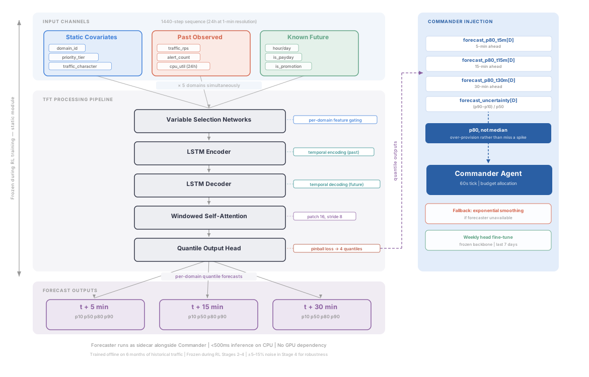
Variable Selection Networks are one of TFT’s most useful features here. They learn, per domain, which input channels matter. For the Payment Processing domain, the variable selection network learns to weight is_payday_flag and is_promotion_flag heavily: payday cycles and merchant promotions are the dominant drivers of payment traffic spikes. For Fraud Detection, it learns that payment volume forecast matters much more than any external event flag; fraud traffic is derived, not independent. The model figures out which inputs matter for each domain on its own — no manual feature engineering.
The quantile output head produces the probabilistic forecasts. Rather than predicting a single value at each horizon, the model predicts multiple quantiles simultaneously, trained with the pinball loss function. The result: a p80 forecast calibrated to be exceeded only 20% of the time, across the entire validation distribution.
What Gets Injected Into the Commander’s Observation
Not all the model’s outputs go to the Commander. I inject:
# Per domain, three horizons
# (shown here with descriptive names; the feature store uses shorter keys):
traffic_forecast_p80_t5m[D]    # 5-min ahead, 80th percentile
traffic_forecast_p80_t15m[D]   # 15-min ahead, 80th percentile
traffic_forecast_p80_t30m[D]   # 30-min ahead, 80th percentile

# Uncertainty signal:
forecast_uncertainty[D]        # (p90 - p10) / p50 at t+15m
                               # normalized ratio, higher = less certain
The forecaster operates at domain granularity because the Commander does — five forecasts per tick, one per domain. Soldiers never see raw forecasts; they receive the Commander’s budget allocation, which encodes the forecast information indirectly. A Soldier handed the raw forecast would have to re-derive the Commander’s arbitration across four domains it cannot observe.
I use the p80 forecast, not the p50 (median). This is a deliberate risk calibration: I would rather pre-provision slightly more capacity than needed than be caught under-provisioned when a spike materializes. The cost of mild over-provisioning is a few extra pods for a few extra minutes. The cost of under-provisioning at this scale is SLO breaches across hundreds of services.
The uncertainty signal (forecast_uncertainty) is equally important. A Commander that ignores forecast uncertainty will treat a high-confidence forecast and a wild guess the same way. The uncertainty signal gives the Commander a reason to request more headroom when the forecast is uncertain. The reward function does not explicitly reward uncertainty-responsive behavior — instead, the Commander learns indirectly that ignoring high uncertainty leads to SLO breaches and the penalties that follow. The forecast_proactivity_bonus pays out on forecast spikes; uncertainty enters only through the SLO penalty. The two interact: a spike forecast with high uncertainty demands a larger budget cushion to avoid that penalty.
The Feedback Loop Trap: Why I Froze the Forecaster
Early in development, I tried training the forecaster jointly with the RL agents. The logic seemed reasonable: as the RL agents learn better scaling policies, the traffic patterns they observe should change (better scaling → rarer latency events → fewer retry storms → lower observed RPS). Why would the forecaster not learn from this?
It should not. Here is the failure mode:
- Commander scales Domain A pre-emptively based on forecast
- Pre-emptive scaling reduces latency, which reduces client retry storms
- Traffic RPS is now lower than it would have been without the scaling
- Forecaster observes lower-than-forecast RPS, updates to predict lower traffic
- Commander receives lower forecast, scales less aggressively
- Domain A gets under-provisioned, latency climbs, retry storms return
- Forecaster now observes higher RPS again
Step 7 puts the system back at step 1. The forecaster’s training distribution shifts based on the Commander’s actions, which changes the Commander’s actions, which shifts the distribution again. The joint system oscillates rather than converging.
In practice, the oscillation was not obvious. Training loss continued to decrease. The forecaster’s MAPE improved. What I noticed was that the Commander’s scaling actions grew more timid with each training epoch — it was learning to trust forecasts that systematically underestimated traffic, because its own scaling had suppressed the observed RPS. The drift toward under-provisioning never registered as a divergence in the training curves; it only surfaced in end-to-end simulation evaluation.
The fix is strict separation: the forecaster is trained offline on historical data, frozen, and treated as a static oracle by the RL training loop. The design refreshes it weekly with a frozen-backbone fine-tune to handle traffic distribution drift, but this fine-tuning is independent of the RL training.
There is a subtler consequence of the freeze-then-fine-tune approach: forecaster drift. The head moves weekly under that fine-tune, but the RL policies in Stages 2–4 were trained against a frozen forecaster. This means the Commander would encounter a forecast distribution that drifts a few percent per week — enough to accumulate meaningful calibration shift over a month — and that it never saw during training. I mitigate this with Stage 4 domain randomization — adding ±5–15% noise to forecast outputs during training so the Commander tolerates calibration shifts. If head fine-tuning drifts beyond that randomization range, the RL policy needs re-fine-tuning.
Edited September 2026: an earlier version described the weekly fine-tune as running in production. It is part of the design, like everything else in this series.
I am not fully satisfied with this answer. The feedback loop problem is real, but freezing the forecaster means it could never learn from what the RL system does downstream of it, and that feels like leaving information on the table. There is probably a way to do safe joint training with the right lag structure or causal separation. I have not found it yet, and destabilizing a payments cluster is not the experiment I would run to find out.
Calibration, Not MAPE
Most time-series forecasting papers optimize and report MAPE or RMSE. Neither helps when the Commander needs calibrated quantiles to make budget decisions.
I care about quantile calibration: does the p80 forecast actually get exceeded 20% of the time?
That one number decides whether the Commander’s budgets are honest. Exceeded 40% of the time, and every allocation it makes is under-provisioned. Exceeded 5% of the time, and I am buying capacity nobody needs.
Aggregate calibration across domains came out close to target, and for a while that was the number I trusted. It was concealing something, and how I found that out is a story for a later post. Once I validated domain by domain and slice by slice, the drift was worse than I expected. Steady-state weekday traffic came out close to target. Weekend patterns were under-confident — intervals so wide that p80 was exceeded under 10% of the time — while event-driven spikes were over-confident, with p80 exceeded closer to 35%.
I fixed this with post-hoc recalibration using conformal prediction — it wraps the model and provides approximate coverage guarantees that the quantile intervals hold on new data, regardless of the underlying model architecture. The recalibration is applied per domain, per time-of-day slice, so the Commander gets calibrated uncertainty no matter the hour.
After recalibration, the p80 forecast is exceeded 18–22% of the time across domains during steady-state traffic — close to the target 20%. During spike events, coverage degrades to 25–30% exceedance, which is acceptable given that the Commander compensates with higher headroom when uncertainty is high. Steady-state MAPE at the 15-minute horizon runs under 10%; spike event MAPE is under 25%. The numbers are good enough for the Commander to act on, and the uncertainty signal tells it when to trust them less.
The forecaster is most valuable during anomalous traffic events, but anomalous events are exactly what it is worst at predicting. It earns its keep on the predictable patterns instead (diurnal ramps, weekly cycles, scheduled promotions). For true black swans, the fallback to conservative over-provisioning is the best it can do.
There is a failure mode worse than high uncertainty: a confidently wrong forecast. This happens when the model predicts a steady-state pattern with narrow confidence intervals, but an unscheduled event — an unannounced merchant flash sale, an upstream service outage generating retry storms — causes traffic to diverge sharply from the prediction. The Commander sees low uncertainty and scales conservatively, right when it should be scaling aggressively. I handle this reactively: the Soldiers detect the SLO breach in real time and can exceed the Commander’s budget by up to 10% to push emergency replicas. If that is not enough — if the forecast was wrong by more than what 10% budget overshoot can cover — the graduated rollback triggers kick in: freeze RL actions, revert to HPA, let the proven reactive controller handle it until the system stabilizes. It works, but it is the least elegant part of the system. The proactive layer fails silently, and the reactive safety net catches it.
Serving Infrastructure
The forecaster runs as a sidecar container alongside the Commander. On each 60-second tick, it pulls a 1440-step input sequence — 24 hours at 1-minute resolution — and assembles known future covariates (calendar events, deployment flags, time context). Inference produces quantile forecasts across all five domains in under 500ms on CPU; no GPU dependency. To hit that budget at this sequence length, I replaced TFT’s temporal attention layer with a windowed variant (patch size 16, stride 8). The forecasts are cached and injected into the Commander’s observation before its own inference runs.
If the forecaster service is unavailable, the Commander falls back to exponential smoothing inline. Less accurate, but always available. An RL agent that silently degrades to bad inputs is worse than one that explicitly falls back to a simpler model.
The forecaster gives the system sight. What it does with that sight depends on the reward function — and getting the reward function right turned out to be the hardest part of the whole project.